15-Minute from Hourly Data

On June 14, 2024, a reform of the balancing market in Poland came into effect. One of the changes is the introduction of a 15-minute energy settlement window, replacing the current hourly one. For energy market analysts, this may present several challenges, such as how to create projections of prices or energy demand with 15-minute granularity based on hourly data.

Various interpolation methods can be used to increase data resolution. In the case of time series, splines are the best suited. Which methods yield the best results? In this article, I examined the following interpolations:

• constant, i.e., assuming the value from the nearest node,
• linear,
• quadratic,
• natural cubic spline, and
• some variations of cubic interpolation, such as Akima, Hermite (Catmull-Rom), Kochanek-Bartels, Steffen, and Steffen’s soft interpolation.

Data Scope, Verification Method, and Error Measure Selection

For the analysis, I selected the values published in 15-minute resolution in the BPKD (current daily coordination plan) by Polskie Sieci Elektroenergetyczne (#PSE) from June 14 to August 25, 2024. First, I intentionally made the data sparser, i.e., aggregated it to hourly data (assuming that the representative value is the average of the four quarters of each hour and assuming that this value applies exactly at the 30^th minute of the hour), and then disaggregated it into 15-minute intervals using the tested interpolation algorithms. Finally, I compared the interpolation results to the original values and calculated the interpolation errors for each method.

As the error measure, I used the Mean Absolute Percentage Error (MAPE):

MAPE = |F – A| / A

where F is the value obtained from the interpolation algorithm, and A is the actually observed (published) value. Naturally, this measure could only be used for those values that do not take on zero or near-zero values, such as:

• KSE power demand,
• planned limitations of availability and withdrawals of MWE,
• sum of generations of scheduling units in the KSE (JGw, JGm, JGz & JGa),
• sum of generations of scheduling generating units (JGw),
• total generation of generating units not actively participating in the balancing market,
• total generation capacity of scheduling generating units (JGw1),
• sum of generation capacities of generating units in the KSE (JGw, JGm, JGz & JGa),
• reserve power capacity over demand,
• reserve power capacity below demand.

Where zero values occurred, I modified the error measure so that the reference point was the maximum value observed during the period:

MAPE = |F – A| / S

where F and A have the same meanings as above, while S represents the maximum observed value during the period, respectively for the following quantities:

• sum of production capacities of energy storage scheduled units  (JGm1),
• total generating capacity of storage scheduling units (JGm1),
• total generation of photovoltaic sources,
• total generation of wind sources,
• total JGm charging power.

Interpolation Error Results

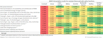
A quick glance at the animated sample chart for KSE power demand on June 20, 2024, is enough to immediately rule out quadratic interpolation among the considered algorithms. However, for the sake of completeness, I have provided results for all methods below—marked in red are the worst, in green the best:

The price we pay for the continuity of the derivative is disproportionately high relative to the obtained results, as illustrated by the following chart for a selected day:

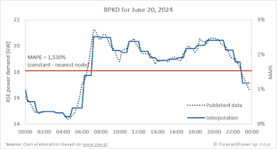
After excluding quadratic interpolation, the weakest results come from constant interpolation from the nearest available node:

This is not surprising—constant interpolation essentially assumes that in every quarter of the hour, we have the average value from the four quarters:

Its use is justified only when we are certain that the original data is indeed hourly (as is currently the case with the national cross-border exchange balance in the BPKD), which means that interpolation is not actually needed.

Linear interpolation, despite its simplicity, performs quite well compared to constant interpolation. However, with few exceptions, its results are mostly inferior to those of cubic interpolations:

Nevertheless, it is worth considering for an obvious reason—it is exceptionally easy to implement.

The comparison of cubic methods looks as follows (colors have been rescaled to reflect the updated range of error values):

Here, the results are not as clear-cut and may depend on the interpolated quantity. On average, Steffen’s two methods and Akima’s method perform best. The cubic natural functions yield slightly worse results, likely due to the failure to meet the monotonicity condition of the interpolation function between the nodes, as a result of the requirement for the continuity of the second derivative at the nodal points.

To select the optimal method, one could also use, for example, a ranking for each analyzed quantity:

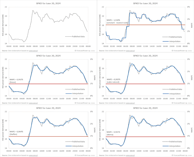
With this approach, Steffen’s smooth method also proved to be the best, followed by Akima’s and Hermite’s methods. Below are visualizations of the results for these three algorithms for the selected day of June 20—this day was characterized by the greatest dispersion of results among these methods (for this particular day, Akima’s method gave a slightly better result than Steffen’s smooth method, which was generally better for the entire data range):

Returning to the MAPE value tables, it is worth noting that the interpolation results for power reserves are much worse than those for other quantities published within the BPKD. Therefore, the reserves are not shown on the histogram below to avoid distorting the scale for the remaining quantities:

The weaker interpolation results for reserves are related to the fact that they can change abruptly from quarter to quarter. For example, for the same day of June 20, 2024, several such sharp fluctuations occurred between 18:00 and 20:00:

Therefore, the interpolation error results for both reserves fall within a much higher range, as illustrated by the histogram below:

Summary

The interpolation results from hourly values to 15-minute intervals of the quantities published within the BPKD using spline functions vary depending on the interpolation algorithm. The best results in terms of MAPE were obtained with modified cubic functions, but they are quite challenging to implement. Slightly worse results were given by natural cubic splines—probably due to the failure to meet the condition for the monotonicity of the function between the interpolation nodes. Fairly good but noticeably weaker results are given by linear interpolation, although it is very simple to implement. Constant interpolation, compared to cubic and linear interpolation, gives much worse results, while quadratic interpolation should be rejected outright.

The results may also vary depending on the interpolated quantities, which is a natural consequence of their variability. When there are significant fluctuations within an hour (as with available power reserves), the interpolation results will be significantly worse. However, regardless of the type of quantities considered above, cubic methods consistently yielded the best results.

Acknowledgement

In determining the interpolated values, I used algorithms implemented in the ACQ library (https://github.com/ratesquant/ACQ). I sincerely thank its authors for creating and sharing it.